










1. Introduction: Why Frequency + Blind Zone + Crosstalk Decide AGV Obstacle-Avoidance Reliability
For AGVs, “seeing an obstacle” isn’t enough—what matters is whether the system can detect it early and consistently, especially in the near field where the safety margin is smallest. In practice, obstacle avoidance performance is often limited less by the sensor’s headline range, and more by three fundamentals:
- Working frequency (e.g., 40 kHz, 48 kHz, 55.5 kHz)
- Blind zone (the minimum distance where reliable detection may be unavailable)
- Crosstalk / mutual interference (how multiple ultrasonic devices can disturb each other)
Choosing the right frequency affects not only echo characteristics and signal-to-noise behavior, but also how well the system supports stable detection under real conditions such as varied target surfaces, installation geometry, and dynamic motion. That is why designers compare options like 40kHz, 48kHz, 55.5kHz e 58kHz ultrasonic waterproof transducer automotive reversing radar when they need reliable obstacle detection for different distance and coverage requirements.
Just as important is the blind zone. Ultrasonic transducers require time to ring down after transmission, and the resulting near-field region can lead to “late” or missing detections if the AGV approaches faster than the system can respond. When blind zone is misunderstood—or when installation height and beam coverage don’t align with the obstacle envelope—operators may observe the same frustrating pattern: the sensor works well at mid distances, but fails right where it should be the most protective.
Finally, AGVs rarely operate with just one ultrasonic channel. In busy warehouses or multi-AGV environments, crosstalk can cause jitter, false alarms, or sporadic missed detections. Even when each sensor is individually accurate, their simultaneous operation can produce confusing echoes. This is why a robust obstacle-avoidance strategy must treat crosstalk as a design constraint, not an afterthought.
In this guide, we’ll walk through how to evaluate frequency selection, interpret blind zone and beam coverage, and implement practical crosstalk suppression approaches so your AGV’s near-distance safety is stable—not just on the bench, but on the floor.
2. AGV Ultrasonic Obstacle Avoidance System Modules
An AGV ultrasonic obstacle-avoidance system is usually built as a signal chain: it emits ultrasonic energy, listens for echoes, converts them into distance/presence information, and then turns that information into safe control actions. Depending on the product design, parts of the chain may be handled externally (e.g., with discrete electronics) or internally (e.g., integrated sensors).

2.1 Transmitting Side: Drive Pulses / Energy Injection
The system starts with an ultrasonic transmit stage that generates short bursts at the target working frequency (commonly in the 40 kHz / 48 kHz / 55.5 kHz / 58kHz family). The output power and pulse timing strongly influence how reliably the sensor can “wake up” an echo from nearby obstacles—especially when the AGV is moving and the geometry changes quickly.
2.2 Receiving Side: Echo Detection & Signal Chain
After the transmit burst, the system switches to a receive function: it captures the returning echo and measures it through a front-end signal chain (amplification, detection, and sometimes envelope processing). This stage determines whether echoes are strong enough to be interpreted as valid obstacle reflections rather than noise, ring-down artifacts, or weak reflections.
2.3 Calculation & Decision: Distance, Thresholds, Filtering, Output
Raw echoes aren’t directly usable for motion control. The system typically performs:
- Distance / presence estimation (often based on time-of-flight principles or equivalent processing)
- Threshold comparison (e.g., warning zone vs stop zone)
- Filtering & stability logic to reduce jitter when echoes vary with target material, angle, or surface reflectivity
- Validity handling (invalid/no-echo cases are treated conservatively so the AGV doesn’t react to unreliable readings)
2.4 Output & Integration: MCU/PLC Interface and Safety Strategy
Finally, the sensing result must be integrated into the AGV’s control layer. The ultrasonic module communicates with an MCU/PLC/controller and triggers appropriate behaviors such as:
- braking / speed limiting
- stop commands
- fault handling or fallback modes when confidence is low
- coordination with other sensors and control loops
In real deployments, this integration layer is where “system reliability” becomes measurable—because the controller’s interpretation of the sensor output directly affects how often you see false alarms, missed detections, or unstable motion.
A key implementation distinction: Transducers vs Integrated Sensors
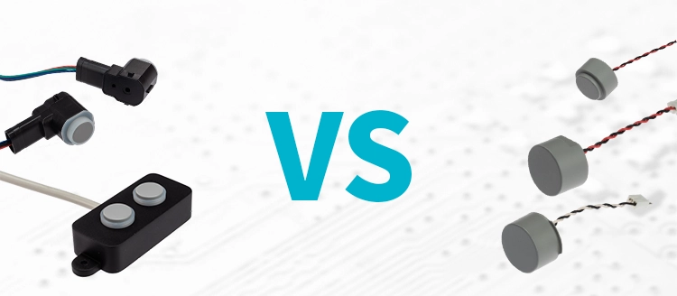
You can also frame the module breakdown based on hardware style:
- Transducer-based products focus on the acoustic front-end. In that case, the AGV system must provide or support the drive/receive circuitry and echo processing, such as with a 40kHz high sensitivity ultrasonic ranging and obstacle avoidance transducer.
- Integrated sensor products include internal signal processing and provide ready-to-use outputs (often analog/digital), allowing faster system integration—commonly exemplified by an AGV obstacle avoidance sensor 1m dual angle.
This distinction matters because it changes where you handle blind-zone behavior and where you implement strategies like crosstalk mitigation and decision filtering (we’ll cover those deeper in later sections).
3. 40kHz vs 48kHz vs 55.5kHz vs 58kHz: Selection Logic & Engineering Trade-offs
When choosing an ultrasonic frequency for AGV obstacle avoidance, the goal isn’t to pick the “highest” number—it’s to pick the option that best matches your required detection distance segment, coverage behavior, and robustness against interference. In near-field avoidance, even small differences in how echoes form and how stable the receive signal is can translate directly into different false-alarm / missed-detection patterns.
Below is a practical way to think about 40 kHz, 48 kHz, 55.5 kHz and 58 kHz—first by clarifying what each design needs to satisfy, then by describing how frequency tends to affect performance directionally, and finally by using a scenario-based selection table.
3.1 Dimensions to Map to Your Requirements
a) Required detection distance range & response speed
In AGV applications, the system must reliably detect obstacles early enough to trigger braking or speed reduction. Your sensing cycle time and echo interpretability matter more when the vehicle is moving quickly and obstacles appear suddenly.
b) Coverage range / “resolution” needs
“Resolution” in ultrasonic ranging doesn’t mean the same as optical pixels, but the practical effect is similar: at the same geometry, different frequencies can influence echo clarity and how consistently the sensor distinguishes between near objects and edge-of-beam reflections.
c) Environment impact & anti-interference priorities
Warehouses and outdoor yards introduce reflectivity variation (metal, concrete, painted surfaces), background noise, and multi-sensor situations. If you plan multi-probe placement, frequency choice becomes part of your broader plan to reduce crosstalk / mutual interference stability issues.
3.2 How Frequency Typically Affects Performance
Rather than relying on a single “frequency → distance” claim, it’s more useful to understand the direction of impact:
- Echo behavior and energy coupling: Higher-frequency ultrasonic signals often have different transducer coupling and echo response characteristics. This can change how easily you get a strong, interpretable reflection from an obstacle at the target distance.
- Signal-to-noise margin: The receive chain depends on echo strength. Frequency selection influences how robust the system can be across varying target materials and installation angles.
- Stability under real geometry: AGV mounting, beam coverage, and the vehicle’s motion can make some frequencies easier to keep stable in borderline conditions (e.g., partial edge coverage, cluttered reflections).
That’s why “reliability-first” selection usually looks like: choose the frequency family that best supports consistent echo interpretation for your specific mounting/coverage plan, then validate blind-zone behavior with test data.
To ground the idea in product categories, you’ll typically see frequency-targeted device lines such as:
- 40kHz ultrasonic ranging obstacle avoidance transducer when you prioritize a common ultrasonic ranging/avoidance tuning approach,
- 48kHz ultrasonic transceiver waterproof obstacle detection when you need an integrated transceiver style with an emphasis on obstacle detection stability under harsh mounting or environmental exposure,
- 55.5kHz ultrasonic ranging transducer safe obstacle avoidance when you want a higher-frequency ranging tuning aimed at safe obstacle avoidance behavior,
- 58kHz ultrasonic waterproof transducer automotive reversing radar when the design focus is similar to automotive reversing radar robustness in real-world conditions.
3.3 Scenario-Based Decision Table
Use the table below as a starting point. After selecting a candidate frequency, you still validate blind zone and coverage geometry on your AGV, because the final reliability outcome is system-level.
| Scenario features | Recommended frequency family | Focus on installation / parameters |
|---|---|---|
| You need robust near-to-mid obstacle detection and a straightforward avoidance tuning approach | 40kHz (often) | Mount height/tilt, beam coverage continuity; validate near-field blind zone and echo stability |
| You want an “obstacle detection” style with integrated transceiver behavior and environmental robustness | 48kHz | Receiver stability across surfaces; waterproof mounting constraints; confirm crosstalk behavior with multi-probe cycles |
| You prioritize safe obstacle avoidance with careful ranging behavior (especially where geometry changes quickly) | 55.5kHz | Confirm that your target obstacle envelope stays inside effective coverage; verify edge-of-beam reliability and threshold settings |
| Your deployment resembles “radar-like” reversing robustness requirements in outdoor/variable conditions | 58kHz (often) | Environmental exposure, waterproof behavior, consistent echo interpretation under different reflectivity targets |
Where the anchor keywords fit naturally in selection:
- If your spec leans toward a classic ranging/avoidance tuning, you may start from 40kHz ultrasonic ranging obstacle avoidance transducer.
- If you need a transceiver concept with stronger emphasis on practical obstacle detection reliability, 48kHz ultrasonic transceiver waterproof obstacle detection is a common direction.
- For safe obstacle avoidance ranging behavior, 55.5kHz ultrasonic ranging transducer safe obstacle avoidance aligns with that goal.
- For “automotive radar” style reversing robustness thinking, 58kHz ultrasonic waterproof transducer automotive reversing radar is a useful reference point.
4. Blind Zone: What It Is and Why It Matters for AGV Obstacle Avoidance
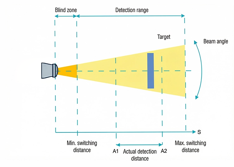
In ultrasonic obstacle avoidance, the blind zone (blind area) is the region where the sensor cannot reliably “see” obstacles. It’s not just a single number like “minimum distance.” For AGVs—where the vehicle moves and the geometry changes quickly—the blind zone can become a real reliability gap: the system may have enough sensing range on paper, yet still miss obstacles in practice.
4.1 Definition & Common Misconceptions
Blind zone is best understood as the combination of:
- Acoustic/receiver limitations near the transducer
Immediately after transmitting, the transducer and electronics need time to settle (ring-down). During this period, returning echoes are hard to detect consistently, so very-close objects may not produce a valid measurement. - Beam coverage and installation geometry
Even when an obstacle is within the sensor’s “nominal range,” it may not be inside the effective acoustic coverage region due to mounting height, tilt, or lateral position. In that case, echoes may be weak or inconsistent—so the system behaves as if it’s “blind” there.
Common misconception: “Blind zone = only minimum distance.”
In AGVs, the blind zone is more like a coverage reliability hole created by both electronics timing and acoustic geometry. That’s why you can sometimes observe different outcomes on straight approaches versus when turning—even with the same sensor hardware.
4.2 Typical AGV Failure Modes Caused by Blind Zone
When blind zone effects show up, they don’t always look like a simple “miss.” Typical AGV behaviors include:
- Straight-line approach: near-field missed detection
The AGV advances and the obstacle enters the near region where echoes are unreliable. The avoidance logic may only trigger after the obstacle is already closer than expected, leading to late braking or abrupt reactions. - Turning: side-front / side-edge leakage
As the AGV rotates, the relative angle between sensor beam and obstacle changes. The obstacle can drift into a region where the beam coverage is less effective, and the blind zone becomes “direction-dependent,” causing side gaps even when forward detection seemed fine during test runs. - Multi-probe cooperation still leaves a local void
Even if you install multiple ultrasonic units, coverage can still have an overlap mismatch—especially when sensors are mounted with slight height/tilt differences or when obstacles appear at specific heights. The result is a local empty region where no sensor has both (a) usable echo timing and (b) sufficient coverage geometry.
This is also where engineers often realize that “range” is not the same as effective coverage, and that blind zone needs to be handled as a system-level design variable—not just a datasheet parameter.
4.3 Strategies to Reduce Blind Zone Impact (Checklist)
A practical way to minimize blind zone risk is to treat it as a coverage engineering problem. Here are the most effective levers:
- Install position & tilt/angle
- Choose a mounting height and inclination that keep the near-field coverage aligned with where obstacles realistically appear on the AGV’s path.
- Avoid designs where the beam “dives” too steeply into the near region or points too far outward, leaving a hole during motion.
- Use more than one probe, and cover multiple directions
- Don’t rely on a single sensor to cover everything. Multi-probe layouts should be planned so that as the vehicle moves and turns, at least one sensor remains in reliable coverage.
- Pay attention to overlap: the goal is to eliminate coverage voids, not just to increase the number of sensors.
- Prefer coverage strategy over single-point dependence
- Combine positioning decisions with validation testing (especially straight approach + turning scenarios).
- If your application requires robust near-field avoidance, a dual-angle concept can be helpful because the beam has different effective angles in the X-plane vs the Y-plane (a “flattened cone” beam), which improves continuous echo coverage across different approach geometries—e.g., designs like 58kHz dual angle ultrasonic obstacle avoidance sensor 1m.
- Select sensor style that fits your integration reality
- For robotics integration, systems often benefit from predictable output behavior and straightforward mounting considerations—commonly seen in products positioned as ultrasonic distance sensor for robotics and smart bins.
5. Beam Angle (Beam Coverage) & Geometry: How to Reduce “Geometry-Based Misses”
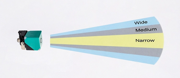
In AGV ultrasonic obstacle avoidance, blind zone often gets the most attention—but many real “misses” happen because of coverage geometry. Even when an obstacle is within the sensor’s nominal range, it may fall into an area where the echo is weak, unstable, or inconsistent due to how the acoustic beam is shaped and how the sensor is mounted.
So in this section, we’ll focus on one key idea:
avoidance reliability = (acoustic reach) × (effective coverage geometry).
5.1 Limitations of a Single-Probe Conical Coverage
Most ultrasonic sensors emit a conical beam. This creates predictable advantages in the center, but it also introduces edge effects:
- Edge reliability decreases
Near the beam boundary, the reflected echo can change rapidly with small shifts in obstacle position (lateral movement, height differences, slight AGV rotation). That’s why the “same obstacle” might trigger avoidance in one approach angle and not in another. - Echo variation depends on obstacle height and shape
For example, a flat plate obstacle vs. a rounded or partially reflective surface can produce different reflection strength at the same distance, especially when the obstacle is not centered in the beam. - Geometry can turn into “direction-dependent blind spots”
A vehicle moving forward with the obstacle near the centerline may be detected well, but when turning (or when the obstacle appears slightly to the side), it may drift toward the beam edge. Then the system can behave like there’s a local blind area—even though the obstacle is “within range.”
In practice, these geometry issues often look like: “It works in the test lane, but fails during real driving paths.” That’s usually a beam-angle and installation-geometry mismatch.
5.2 Why Multi-Angle / Wide Coverage Helps
A straightforward way to reduce geometry-based misses is to increase coverage continuity rather than relying on a single conical region.
- Dual-angle comes from beam shape (not necessarily two probes)
Assuming the transducer’s emission axis is along the Z-axis, the ultrasonic energy forms a conical beam, but its effective width is not identical in the X and Y directions. This creates a “flattened cone” (elliptical beam): the effective half-angles differ between the X-plane and the Y-plane, which is why it’s called dual angle. This asymmetric beam geometry improves continuous coverage and reduces edge-related missed detections as the AGV transitions from straight motion to turning. - Better matching between left/right coverage and front coverage
In AGV setups, “what matters” changes with movement:- during forward travel: front-left and front-right angles both matter,
- during turning: side-front geometry matters even more.
This is why you’ll often see product lines positioned around dual-angle coverage, such as AGV obstacle avoidance sensor 1m dual angle—they’re designed to make the coverage behave more consistently across different approach geometries.
Additionally, for robotics platforms that need predictable integration behavior (mounting, wiring, signal stability), teams frequently choose sensor modules like ultrasonic distance sensor for robotics and smart bins where the system can be tuned around a clear output behavior rather than “guessing” the detection pattern from raw acoustic performance.
5.3 Turn Beam Angle Into Installation & Acceptance Testing
To truly minimize geometry-based misses, you should translate beam angle into a measurable acceptance process, not just a mounting guideline.
Cover validation steps (recommended):
- Test obstacle heights and materials—not only distances
Use at least a couple of obstacle heights relevant to your AGV (e.g., bumper-level and lower/higher forms). Material reflectivity matters because it affects echo strength and stability at the beam edges. - Map coverage at multiple lateral offsets
During tests, place the obstacle slightly left, centered, and slightly right relative to the sensor direction. This quickly reveals whether detection is stable near beam boundaries. - Verify during motion modes (straight + turn)
Geometry problems often show up during turning. Plan scenarios where the AGV rotates at realistic angles and speeds, and confirm that the avoidance trigger remains consistent.
Record and iterate:
After each test run, document:
- sensor mounting angle/tilt,
- obstacle relative position (left/center/right and height),
- whether echoes produce stable outputs (not just “a reading exists”).
Then adjust installation and/or choose a coverage strategy that reduces the probability of obstacles landing in weak-echo zones.
6. Multi-Transducer Crosstalk & Mutual Interference: Why AGV Gets “Less Stable” After Installing More Sensors
Once you move from one ultrasonic channel to a multi-probe layout, a new reliability threat appears: crosstalk / mutual interference. In real AGV environments, this is a common reason you’ll see distance jitter, occasional false alarms, or even missed detections—especially during turning or when multiple vehicles operate in the same area. Crosstalk is also widely recognized as a major cause of wrong distance measurements in mobile robots when sonar/ultrasonic transducers interact.
The core reason is simple: ultrasonic signals can overlap in space and time, and one sensor may inadvertently detect echoes that were generated by another sensor (or its transmit/settling artifacts).
6.1 Common Crosstalk Symptoms
Look for patterns like these:
- Distance jumps & jitter
The measured distance rapidly changes between two values even when the obstacle hasn’t moved. - Occasional false alarms / leakage into decision logic
The system triggers avoidance unexpectedly (e.g., “stop” when the path is clear). - Occasional missed detections
The opposite can also happen: a valid obstacle echo is masked or the system discards it due to inconsistent readings. - Worse during turning / multi-vehicle scenarios
Turning changes relative geometry, so reflections and overlap conditions shift quickly. In multi-AGV environments, simultaneous operation can increase interference probability.
6.2 Engineering Methods to Suppress Crosstalk
Crosstalk mitigation is typically a layered strategy—don’t rely on only one measure.
1) Time / multiplexed (time-sliced) firing
Instead of letting multiple sensors transmit freely, coordinate them so that only one (or a controlled subset) emits within each cycle. This reduces the chance that a “receive window” catches another sensor’s transmitted burst.
If your hardware supports synchronization inputs (or you can implement strict software timing), it makes multi-sensor operation significantly more stable by design [ref:4].
2) Use a receive “range gate” concept
Even with controlled timing, echoes from different distances (or from unintended reflectors) can interfere. A range gate approach restricts what you consider valid by only accepting echoes inside an expected time/distance window for each sensor’s intended coverage.
Practically, you define:
- expected near/stop region,
- expected warning region,
- and discard returns outside those gates (or treat them as low-confidence).
3) Installation geometry & shielding
Physical arrangement still matters:
- place sensors with sufficient spacing (or alternate positions),
- avoid orientations
6.3 Quick Troubleshooting Workflow (Phenomenon → Verification → Tuning)
When the system becomes “unstable” after adding probes, don’t guess—follow a structured process:
1. Single-probe validation first
Test each sensor alone in the same environment and log:
- echo stability / presence detection behavior,
- false alarm rate,
- and repeatability of the decision output.
2. Then compare dual-probe behavior
Add a second sensor and repeat the same tests. Focus on:
- which direction causes the jitter,
- whether the false alarms correlate with certain obstacle positions.
3. Finally test multi-probe / full deployment
Turn on the full array and verify:
- stable avoidance triggers across straight and turning paths,
- stability at the edges of coverage (where ambiguity is highest),
- multi-vehicle interference if applicable.
4. Tune in the right order
- Start with timing/multiplex schedule,
- then range gate windowing,
- then threshold/filter logic,
- and only after that consider frequency mix or installation tweaks.
This “single → dual → multi” sequence prevents you from chasing symptoms without isolating the cause.
7. Transducer vs Integrated Sensor: Integration Boundaries for AGV Systems
When integrating ultrasonic obstacle avoidance into an AGV, one of the most practical decisions you’ll make is whether to work with a transducer-style product (acoustic element + high-frequency electrical characteristics) or an integrated sensor (with built-in signal processing and ready outputs). This choice directly affects how much engineering you do on timing, echo detection, filtering, and how quickly you can reach stable avoidance behavior in the field.
A helpful way to frame it is: transducer-based design shifts more work to your electronics and algorithms; integrated sensors shift more work to the supplier’s internal processing.
7.1 Transducer Type
What you get: mainly the acoustic front-end. You typically receive a device described as a transducer for ranging/avoidance, but the rest of the system—drive waveform, receive amplification, echo detection, and decision logic—must be handled externally.
What this means for AGV integration:
- You usually need external drive circuitry and a carefully designed receive signal chain (amplification, detection, timing).
- You must implement or tune an algorithm that transforms echoes into distance/presence decisions.
- Commissioning often takes longer, because you’ll validate not only placement, but also signal stability across conditions (mounting tolerances, obstacle materials, and multi-probe interactions).
If your development team has the capability to design and tune that end-to-end chain, transducer options can be a strong fit. For example, in product terms you may encounter transducer references like:
- 40kHz high sensitivity ultrasonic ranging and obstacle avoidance transducer
- 40kHz ultrasonic reversing radar transducer high sensitivity reliable obstacle detection
- 48kHz ultrasonic transceiver for car reversing collision avoidance waterproof design
- Transdutor de alcance ultrassónico de 55,5 kHz para evitar obstáculos em segurança ao fazer marcha-atrás em automóveis
- 58kHz waterproof ultrasonic transducer for automotive reversing radar systems
Those keywords typically signal the intended use-case (ranging, reversing-radar-like robustness) and hint that you’re closer to building an acoustic subsystem than “plugging in a distance value.”
7.2 Integrated Sensor Type
What you get: the ultrasonic front-end plus internal signal processing. The sensor returns outputs that are directly usable by your controller—often analog or digital signals—so your AGV integration can focus more on mounting, wiring, and decision thresholds than on echo math.
What this means for AGV integration:
- Faster bring-up: you can verify avoidance triggers sooner.
- Less time spent on raw echo handling and signal chain design.
- Easier standardization across vehicles (especially when deploying fleets where uniform behavior is critical).
In product language, integrated sensor options are commonly represented as:
These names often emphasize coverage geometry (“dual angle”) and robotics-friendly integration (“distance sensor”), which aligns with the idea that you’re consuming stable measurement outputs rather than implementing the entire ultrasonic pipeline yourself.
7.3 When to Choose Transducer vs Integrated Sensor
Here’s a practical decision boundary—based less on “which is better,” and more on what you need to control inside your project:
1. System development resources vs. delivery timeline
- If you have strong embedded/electronics resources and want flexibility, a transducer-based approach (e.g., 40kHz high sensitivity ultrasonic ranging and obstacle avoidance transducer) can support deeper optimization.
- If you need stable obstacle-avoidance behavior quickly, integrated sensors (e.g., ultrasonic distance sensor for robotics and smart bins) reduce integration risk.
2. Interface and control requirements
- Transducers often require more custom interface work (drive + receive + timing + algorithm integration).
- Integrated sensors usually provide easier analog/digital outputs, which simplifies wiring to your MCU/PLC and tuning avoidance thresholds.
3. Engineering maintainability across changes
- With transducers, your behavior depends heavily on your drive/receive tuning choices. Small changes in your electronics or mounting may require re-validation.
- With integrated sensors, many variables are pre-packaged, so your repeatability improves when scaling production.
4. How you plan to address multi-probe behavior (ties back to crosstalk)
- No matter which type you use, multi-probe environments still need system-level mitigation (timing coordination, validation logic, thresholding).
- However, integrated sensors may include more consistent internal processing behavior cycle-to-cycle, which can make multi-probe tuning less “wild” during early trials—so you can get to a stable baseline faster.
8. Field Validation & Acceptance: Make Obstacle Avoidance Reliability Quantifiable
After selecting frequency/coverage geometry and mitigating crosstalk, the real proof comes from field validation and acceptance testing. For AGVs, “works on the bench” isn’t enough—because performance failures usually emerge from the combination of blind zone behavior, beam geometry, multi-probe timing, and real-world obstacle/reflectivity patterns.
The goal of this section is to help you turn avoidance reliability into measurable KPIs and repeatable test cases, so you can compare configurations objectively and close the loop (blind zone → crosstalk → thresholds/filters).
8.1 Test Scenario Design
Design scenarios around how the AGV actually moves and how obstacles appear:
- Forward path
Straight approach toward obstacles at multiple distances, especially entering the near region where the blind zone risk is highest. - Side-front / lateral zones
Obstacle positions slightly left and right of the sensor centerline. This catches “geometry-based misses” that may not show up in straight-line tests. - Turning regions (the highest-stress case)
Run controlled turn maneuvers where relative angles change quickly. Crosstalk and beam-coverage edge effects often become visible during turning.
Then vary obstacle characteristics:
- Different obstacle heights / distance steps
Don’t only test one “bumper-level” obstacle height. Use at least a lower, nominal, and higher height that matches your expected environment. - Typical environmental conditions
Include cases such as dust, rain/fog, and reflective differences (metal vs painted surfaces vs concrete). These can change echo strength and stability, which directly impacts alarm triggering and false alarm behavior.
8.2 Evaluation Metrics
To “quantify reliability,” define metrics that map directly to what can go wrong:
1. Alarm trigger distance stability
- Measure how consistently the avoidance trigger occurs at the intended distance across repeated runs.
- You care about both mean trigger distance e spread/jitter (because jitter can cause unstable speed control).
2. False alarm rate (virtual detections)
- How often the system triggers avoidance when no valid obstacle is in the path/coverage zone.
- In multi-probe setups, false alarms may correlate with specific vehicle angles, obstacle materials, or simultaneous sensor cycles.
3. Missed detections (leak-through events)
- Count cases where an obstacle should have been detected (based on coverage/geometry) but wasn’t.
- Treat this as a safety-critical metric—misses are usually the hardest failures to accept.
4. Multi-probe parallel stability
- Compare behavior with 1 probe vs 2 vs the full array.
- Look for patterns like distance jitter, inconsistent outputs between channels, or decision thrashing during motion transitions.
If you structure your acceptance report around these items, you’ll be able to distinguish “sensor placement is okay but thresholds need tuning” from “coverage still has a void” or “timing causes interference.”
8.3 Tuning & Re-test Closed Loop
Validation shouldn’t be a one-time pass; it’s a closed loop. A practical iteration order is:
1. Blind zone / coverage first
- If you see misses near the near-field or at specific angles, adjust mounting position/tilt and/or improve coverage strategy (e.g., dual-angle coverage, overlap) before touching heavy filtering.
2. Then address crosstalk / mutual interference
- If you see jitter or inconsistent readings appearing after adding probes, focus on multi-probe timing coordination and decision consistency rules.
- Re-test turning and multi-probe overlap scenarios after each change.
3. Finally tune thresholds & filtering
- Adjust warning/stop thresholds so they match the measured trigger stability.
- Apply filtering/consistency logic to reduce jitter, but keep an eye on missed detections—over-filtering can hide real echoes.
4. Repeat targeted test subsets
- Don’t re-run everything blindly. Each iteration should focus on the scenarios where failures were observed (forward near region, side-front edge, turning cases, specific obstacle heights/materials).
9. Conclusion
Reliable ultrasonic obstacle avoidance for an AGV is never just about the sensor’s nominal range. To make the system dependable in real driving, you need to align frequency selection, blind zone behavior, beam angle / coverage geometry, and multi-probe crosstalk suppression into one coherent design—then prove it through structured field validation.
If you’re planning a deployment, a good starting checklist is:
- your target minimum safety distance,
- the obstacle height range you must detect,
- the number of probes and their mounting positions/angles,
- your preferred output interface needs (analog/digital) for MCU/PLC integration.
From here, choose the integration path that best matches your resources and timeline:
- Transducer front-end route: suited when you want more control over drive/receive/echo processing. You can evaluate options like 40kHz high sensitivity ultrasonic ranging and obstacle avoidance transducer or automotive-style references such as 55.5kHz waterproof ultrasonic transducer for automotive reversing radar systems.
- Integrated sensor route: suited when you want faster commissioning with ready-to-use proximity/distance outputs, such as AGV obstacle avoidance sensor 1m dual angle e ultrasonic distance sensor for robotics and smart bins.
FAQ
Q1: Why should AGV obstacle avoidance focus on blind zones instead of only "range"?A1: Because range tells you the theoretical maximum sensing distance, while the blind zone is where echoes can't be reliably detected (due to near-field timing, mounting geometry, and beam coverage). An AGV can therefore behave safely on paper but still miss near obstacles or behave inconsistently when the vehicle moves into turning/side-front geometries.
Q2: How should I prioritize 40kHz vs 48kHz vs 55.5kHz?A2: Treat it as a system-matching exercise:
- Start with your required detection behavior (early warning distance, response urgency).
- Consider your coverage geometry (mount height/tilt, obstacle envelope).
- Then validate robustness in your environment and multi-probe setup.
In other words, don't pick purely by frequency number—pick based on which candidate transducer family gives you the most consistent obstacle decision after installation and tuning. Common starting points you'll see in the market include 40kHz ultrasonic ranging obstacle avoidance transducer, 48kHz ultrasonic transceiver waterproof obstacle detection, and 55.5kHz ultrasonic ranging transducer safe obstacle avoidance.
Q3: If multiple sensors interfere, how can I tell whether it's crosstalk or a mounting problem?A3: A good troubleshooting rule:
- If the "instability" correlates strongly with which sensor transmits/receives in a cycle (and changes when you alter timing/multiplex order), it's likely crosstalk.
- If the issue persists even after timing changes, and especially if it correlates with specific obstacle angles/heights, it's more likely geometry/mounting (beam overlap, tilt direction, or physical obstruction). Also run the "single → dual → multi" validation sequence to isolate the cause.
Q4: How does beam angle affect left/right coverage?A4: Beam angle determines where the echo strength remains stable across lateral positions. Near the beam edges, you may get weaker or more variable reflections, which can make one side detect reliably while the other side becomes intermittent. That's why many designs move from single-beam reliance toward dual-angle coverage strategies—e.g., AGV obstacle avoidance sensor 1m dual angle—to improve continuity during lateral shifts and turning.
Q5: Does dual-angle / multi-direction placement really help reduce missed detections?A5: Yes—when the “dual angle” refers to the elliptical/flattened cone beam (different effective angles in the X-plane vs Y-plane), it improves coverage continuity and makes obstacle echoes more stable across vehicle motion states. It reduces the chance that obstacles repeatedly fall into weak-echo regions as the AGV moves and turns, helping to mitigate the “geometry-based misses” that appear when relative obstacle position changes quickly.
Q6: How do analog/digital output interfaces impact AGV integration?A6: They affect integration effort and stability of control logic:
- Digital outputs can simplify MCU logic and speed up bring-up, but you still need to understand how the sensor decides "trigger vs no trigger."
- Analog outputs can give more information (e.g., distance/proximity magnitude), which can improve filtering and thresholding—useful when the environment is variable.
In practice, integrated solutions positioned as robotics-friendly distance sensors can reduce uncertainty in the signal chain, such as ultrasonic distance sensor for robotics and smart bins.
Q7: Transducer vs integrated sensor: what's the real difference in commissioning cost?- With a transducer-based approach, you typically handle more of the ultrasonic pipeline: drive waveform, receive amplification, echo detection, and algorithm/threshold tuning. That can mean higher engineering time but more flexibility.
- With an integrated sensor, internal processing is handled by the supplier, so you focus more on mounting, timing coordination between probes (if multi-sensor), and system-level thresholds.
If you're building a system quickly or deploying at scale, integrated units like AGV obstacle avoidance sensor 1m dual angle often shorten commissioning time because you get stable outputs sooner.
Q8: What kinds of behavior should I expect when switching between indoor/outdoor conditions?A8: Outdoor environments introduce larger variations: reflective surfaces, dust, rain/fog, and background acoustic clutter. You may see:
- higher false alarm probability if thresholding is too permissive,
- more frequent jitter in the warning region if the received echo is unstable,
- inconsistent performance around specific obstacle materials (metal vs painted surfaces).
That's why field validation should include your realistic environments—not only a single test lane.
Q9: How should I design acceptance test cases?A9: Base them on the failure mechanisms you care about:
- Blind zone / near-field tests (straight approach and slow/fast speed variants).
- Beam geometry tests (left/center/right obstacle offsets; different obstacle heights).
- Crosstalk tests (single probe vs dual vs full array; include turning scenarios and multi-vehicle when relevant). Then define pass/fail KPIs like alarm trigger stability, false alarm rate, missed detections count, and multi-probe parallel consistency.
Q10: How can I verify crosstalk risk when multiple AGVs operate simultaneously?A10: Run a fleet-style test:
- Ensure each AGV uses its ultrasonic system under realistic motion (including turning).
- Observe distance jitter and false alarm patterns correlated to neighboring AGVs.
- If instability increases only when multiple vehicles transmit concurrently, that indicates mutual interference risk.
As a reference for products often marketed for robust operation (including reversing-radar-like durability), you may consider evaluating models such as ultrasonic transceiver 55.5kHz waterproof in your comparative setup—then still confirm that your timing strategy and mounting geometry solve the system-level interference.
Q11: Is there a "best practice" to tune thresholds and filters without hiding real obstacles?A11: Yes: tune with a safety-first approach.
- Start by ensuring the sensor can reliably detect obstacles in the critical near region (blind zone + coverage).
- Then tune warning/stop thresholds to match the observed trigger stability.
- Use filtering to reduce jitter, but validate it won't delay or suppress real detections—especially for lower obstacles and edge-of-beam positions.
-
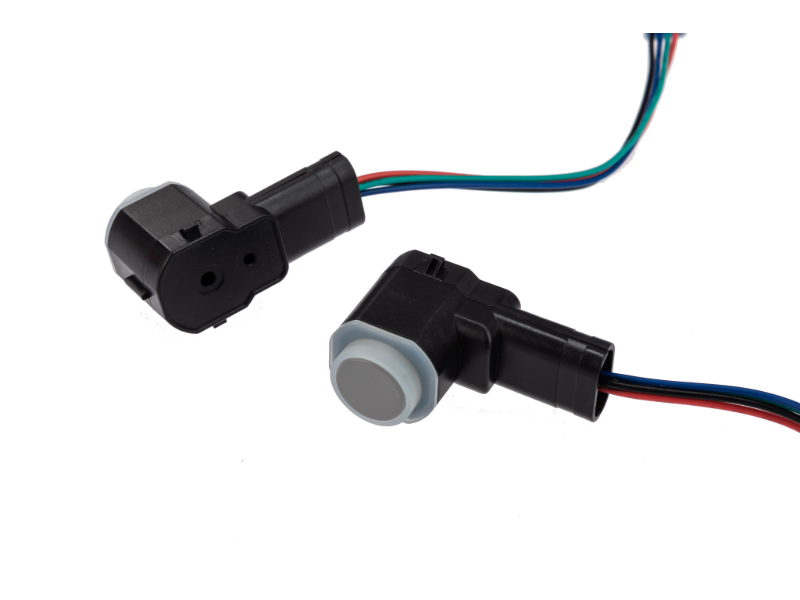
ISSRSensor 1M 58kHz Ultrassónico AGV Sensor de Prevenção de Obstáculos
-

ISSRSensor Sensor de distância ultrassónico 1M 58khz para robótica e caixas inteligentes
-
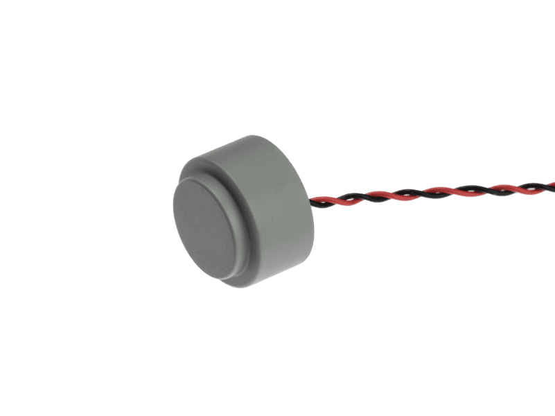
ISSRSensor Transdutor ultrassónico de alta sensibilidade de 40kHz para localização e prevenção de obstáculos
-
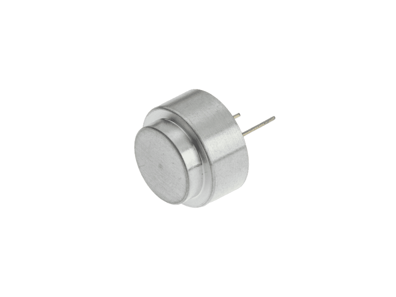
Transdutor de radar ultrassónico de marcha-atrás ISSRSensor de 40 kHz | Alta sensibilidade e deteção fiável de obstáculos
-
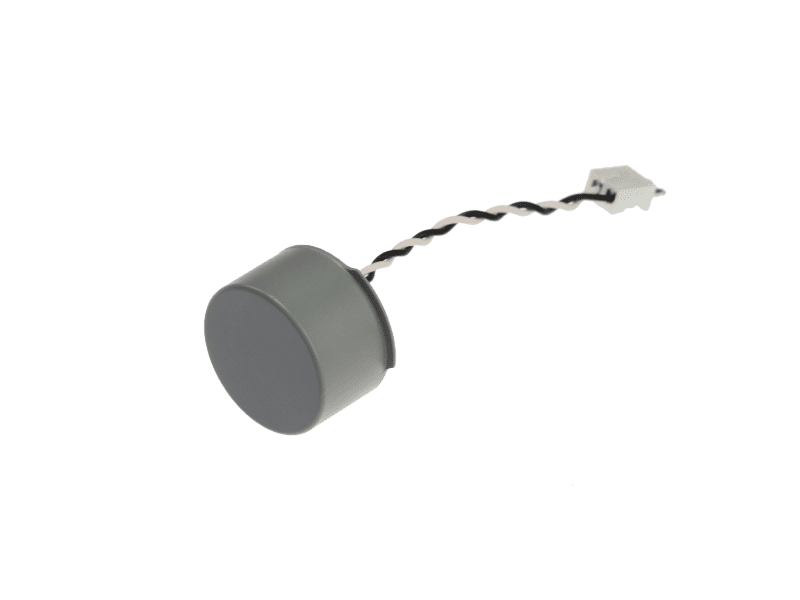
ISSRSensor 48kHz Ultrasonic Transceiver for Car Reversing Collision Avoidance – Waterproof Design
-
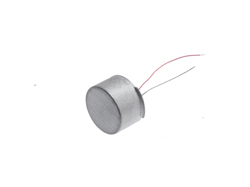
ISSRSensor Transdutor de alcance ultrassónico de 55,5 kHz para evitar obstáculos em segurança ao fazer marcha-atrás em automóveis
-

ISSRSensor Transdutor ultrassónico à prova de água de 55,5 kHz para sistemas de radar de inversão de marcha para automóveis
-
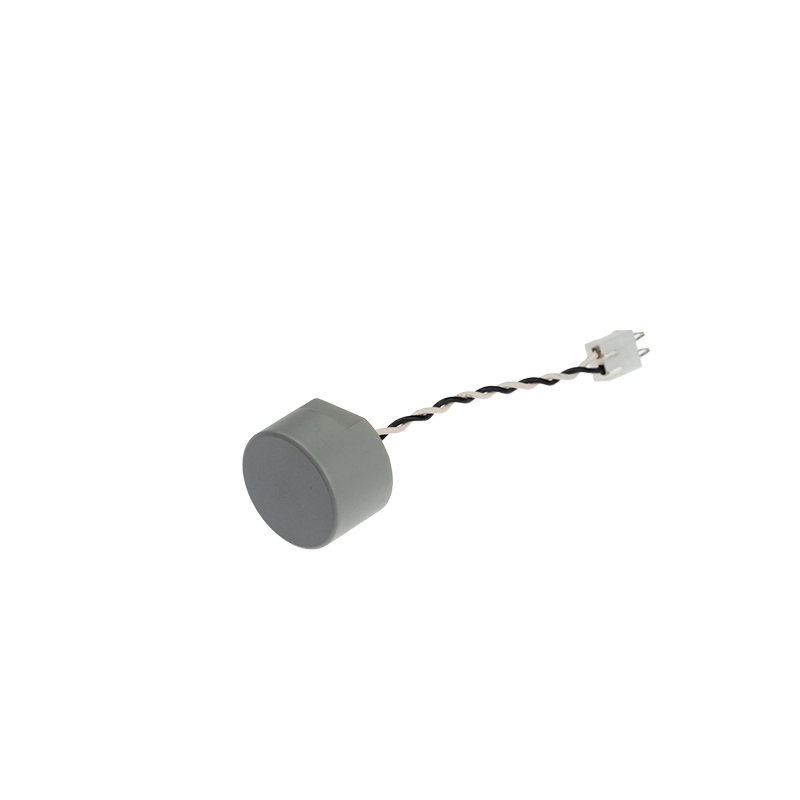
ISSRSensor 58kHz Ultrassónico de Baixa Frequência e Transdutor para Evitar Obstáculos
Entrar em contacto